Zaragoza NLOS synthetic dataset
This website is made for sharing synthetic Non-Line-of-Sight scenes rendered using the publicly available transient renderer from Jarabo et al's work in A Framework
for Transient Rendering
.
The data and tools are still in development so if you have any questions, suggestions or issues, please send us an email to juliom (AT) unizar (DOT) es.
This project is co-funded by the DARPA REVEAL project and a BBVA Foundation Leonardo
grant.
If you use this dataset please add a reference using these bibtex entries.
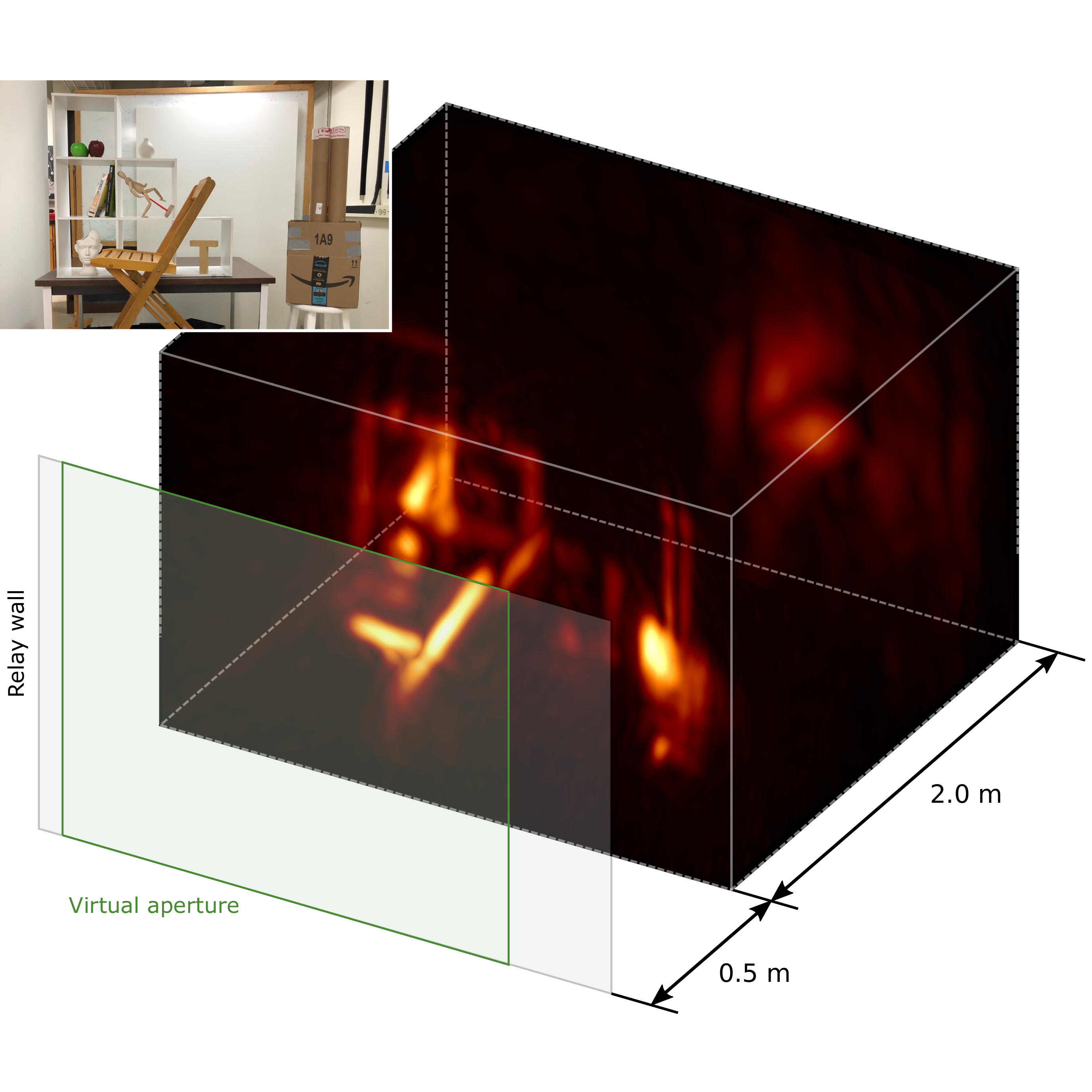
We've added the synthetic scenes from our recently accepted Nature paper Phasor Fields: Virtual Wave Optics for Non-Line-of-Sight Imaging.
Use the text input to filter
for the parameters you want, and click on each row to see the download links. You can also download all the files using the following links:
- Datasets in HDF5 format.
- Scenes in Blender format.
Please send us an email to juliom (AT) unizar (DOT) es if you find any issues.

Scenes
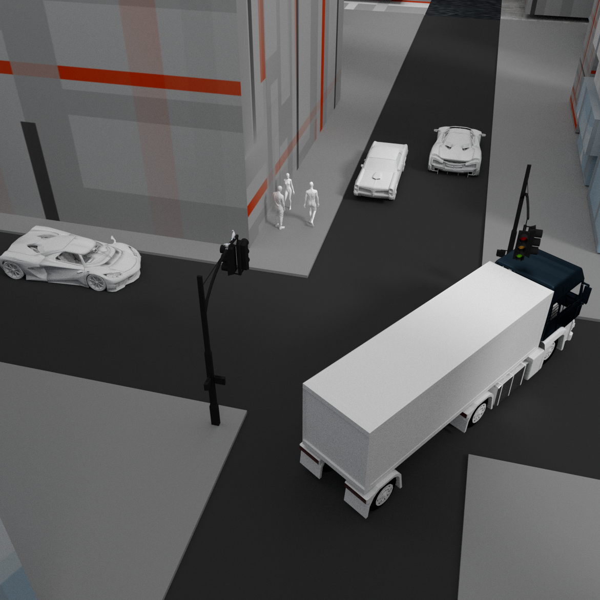
We consider two types of scenes: those following the canonical setup of a single hidden object in front of a diffuse wall (as you can see on the diagram below), and realistic indoor and outdoor scenarios.
A time-resolved sensor in the scene captures the radiance reaching a grid of points on the wall, with part of the scene remaining hidden from its line of sight. Using these simulated captures we can test algorithms to reconstruct
the hidden geometry.
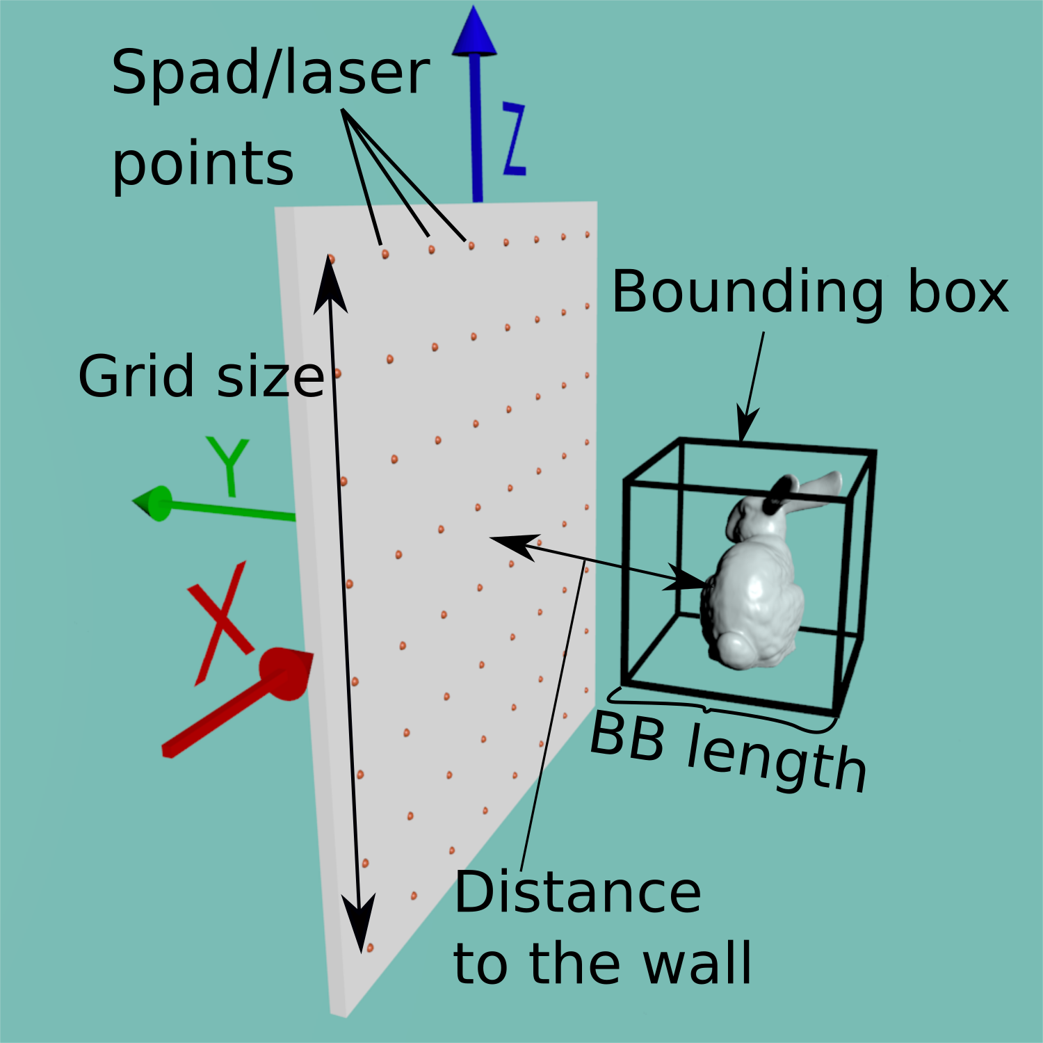
Example setup scene with a floating hidden object.
Complexity
The scenes here are ordered by 'Complexity'. This refers to the ammount of Multiple Path Interference (MPI) that can be expected in the scene.
At this point, we are working with the following levels of complexity:
- Floating: the hidden object floats in front of the wall. There is no interference outside of that occuring within the object and with the wall.
- On the floor: the hidden object is placed on top of a plane. In this case, radiance will reach the sensor coming from both the object and the floor, including paths that followed bounces between them.
- In a box: the object is again placed on top of a plane, but this time completely enclosed within 6 walls. You can expect these scenes to have more MPI than any others, since all paths will find another surface to bounce off of.
- Complex / realistic: There is no strict structure to these scenes. Hidden objects may be appear anywhere, and any surface can act as the relay wall. You may want to reconstruct the whole scene or just parts of it, since they contain many regions of interest.
- Phasor: Synthetic scenes from our newest article.
Hidden objects
These are the hidden objects we've used for the following scenes:
- T: a 3D letter 'T', meant as a simple to reconstruct geometric shape.
- USAF: 2D texture showing rectangles of different sizes. Meant as a way to find the precision of the data and reconstruction system
- Concav: a 3D surface showing multiple concave and convex surfaces. These surfaces are typically difficult to reconstruct due to the MPI occuring within it.
- Bumps: a plane with smooth concave and convex bumps.
- Spheres: two simple spheres placed at two distances.
- Stanford Bunny: a well-known capture of a 3D bunny. Good for showing the precision of the reconstruction.
- Indonesian statue: bust of a person, with smooth and higher-order features.
- Serapis: bust of a person, with smooth and higher-order features.
- Lucy: complex statue of an angel, with very fine details, occlusions and interreflections.
- Chestnut: a chestnut tree. Specially complex due to the interreflections occurring between its leaves.
- Sports car: a smooth, highly-detailed model of a sports car. Its surfaces at an angle make it difficult to reconstruct.
- XYZRGBDragon: dragon with smooth features, concave surfaces and oclusions.
- Chinese: dragon with smooth features, concave surfaces and oclusions.
- Hairball: ball made of strands of hair, very fine details and complex interreflections occur within it.
The 'Bounding Box (BB) length' column on the datasets refers to the length of the sides of a cube bounding the geometry. This is mostly useful for backprojection algorithms that can work on a delimited volume instead of the whole scene, saving time and memory.
Dataset file description
| Field | Description |
|---|---|
| cameraPosition | Position of the SPAD |
| cameraGridNormals | List of capture point normals. Points start at the top left of the grid going to the right and bottom. |
| cameraGridPositions | List of capture point positions. Points start at the top left of the grid going to the right and bottom. |
| cameraGridSize | Width and height of the capture grid. |
| cameraGridPoints | Number of capture points in the grid in X and Y. |
| laserPosition | Position of the laser that generates the virtual point lights in the grid. |
| laserGridPositions | Positions of each virtual point light. Virtual point lights in the grid start at the top left of the grid going to the right and bottom. Since the grid is in a plane they are the same in most cases. |
| laserGridNormals | List of virtual point light normals in the grid. |
| laserGridSize | Width and height of the virtual point light grid. |
| laserGridPoints | Number of laser points in the grid in X and Y. |
| data | Monochrome transient image container. Its size is N_POINTS_X x N_POINTS_Y x BOUNCES x TIME_RES. In a non-confocal setting, the size may be N_LASER_POINTS_X x N_LASER_POINTS_Y x N_SPAD_POINTS_X x N_SPAD_POINTS_X x BOUNCES x TIME_RES. Light bounces are stored separately and should be added together for closest to reality results (or use only the 2nd bounce for best results). Newer data has an extra dimension for color channel, used for testing. It shouldn't matter in most cases since it's a singleton dimension in most cases. |
| deltaT | Time resolution for each pixel on the transient image in distance units. For instance, deltaT=0.001 means each pixels captures light for the time it takes it to travel 0.001m in the scene with c=1m/s. |
| hiddenVolumePosition | Center position of the volume containing the hidden geometry. Useful for backprojection algorithms that only work on a volume. |
| hiddenVolumeRotation | Rotation of a volume containing the hidden geometry with respect to the original geometry. Useful when comparing reconstructions. |
| hiddenVolumeSize | Dimensions of the box that tightly bounds the hidden geometry. |
| isConfocal | True if the data was rendered confocally, that is, the spad and laser grids are the same size, have the same number of points and only the positions where both match were rendered/captured. |
| t | Time resolution. |
| t0 | First instant captured in each transient row. |
3D probability volumes
We work with hdf5 files for the reconstructions and ground truth data. They can be easily compressed and read, and we can include multiple volumes with metadata in a single file.
A single hdf5 file can contain both multiple ground truth and reconstructions with the following structures respectively:
 /position{x,y,z}/size{sx,sy,sz}/ground-truth/voxel-resolution{rx,ry,rz}/voxelVolume
 /position{x,y,z}/size{sx,sy,sz}/reconstruction/rec_method/filter/max_bounce{}/voxel-resolution{rx,ry,rz}/voxelVolume